DOE Other Models

DOE Models: Introducing Box-Behnken Design or BBD

The Bancon Box Design (BBD) model as a DOE model has three levels for dividing design points related to input parameters or factors. Three levels include -1, 0, +1, where levels +1 and -1 are equivalent to the maximum and minimum values of each input parameter, respectively, and level 0 is equivalent to the mean value of that parameter. Therefore, each input parameter is divided into three parts or levels between its maximum and minimum values. Hence, the median level is always equal to the median value between the maximum and minimum values.

The number of divided modes in the present model is obtained from the following equation:

• k represents the number of input parameters or the same factors. According to the following formula, the number 1 illustrates only the case where all factors have their middle value (same as level 0).
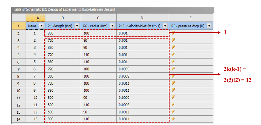
• The expression 2(k(k-1)) represents the states in which, for each parameter, the constant middle value. It is considered with the maximum and minimum values of other parameters (same as level +1 and level -1).

Figure 1 shows the design space for design points in the Bancon Box Design (BBD) model for the mode with two input parameters.

As can be seen from the figure, if we consider two horizontal axes and one vertical axis as a range for selecting design points, we see that the middle value of each input parameter is between the maximum and minimum values of the other input parameter, the other input.

Figure 1. Generating a box Banknote Design for Two Input Parameters

An Example of Box-Behnken Design

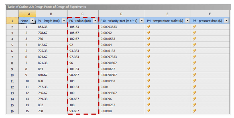
For example, suppose that there are three input parameters or variables, including length, radius, and velocity inlet, as design points. Figure 2 shows a table of creative design points for each input parameter.

Figure 2. Creative Design Points Table in an Example with Three Input Parameters Using the Box Design Method

Comparison between CCD (Face-Centered), CCD (Rotatable) and BBD

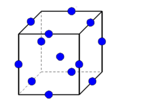
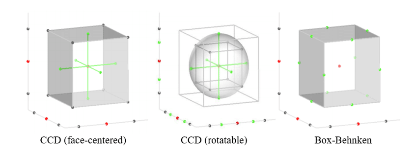
Figure 3 compares design points with three different design methods, including a Face-centered central composite design model and a rotatable central composite design model. And is the design model of Bancon Box (BBD).

In all three design methods, three input parameters or variables are considered. Hence, all three images related to the design point space have three axes containing a range of input parameters.

Figure 3: Distribution of Design Points for the Design Model with three Input Parameters in Different Ways

Advantages of Benken box design method compared to central composite design method:

• It requires fewer design points and, therefore, less computational time.
• The lack of points in the corners of the space for design points allows the user to work well around a combination of input parameters.

Disadvantages of Benken box design method compared to central composite design method:

• Unable to predict the points in the corners of the space for design points.
• Only three levels are considered for each input parameter, which may reduce the accuracy of the prediction.

DOE Models: Introducing the Optimal Space-Filling Design Model

The optimal space-filling design model  as a DOE model divides each input parameter into several parts. This design model is divided according to the number of sample points, and the values ​​of these sample points include different types (sample type).  Also, the number of input parameters or variables in each model determines the number of segmented points.

This model of design has several features:

• The model can distribute design points evenly within the design space.
• This model aims to achieve the most analytical vision using the least number of design points.
• This model can manually adjust the number of design points using auto-defined samples mode. Therefore, this model is very suitable for times when there is a computational time limit.
• The location of design points within the design space is heterogeneous; in this model, unlike previous models, it is not necessary to place design points in the corners or midpoints.

Figure 4 shows the design space containing the design sample points according to the optimal filling space design method. Two input parameters are considered in this design space, divided into five levels.

Figure 4. Distribution of Sample Points in the Optimal Filling Space Design Model with Two Input Parameters

Sample Point Distributions of the Optimal Filling Space Design Model Types

The types of sample point distributions of the optimal filling space design model include the following:

• Central Composite Design (CCD samples)
• Linear model
• Incomplete quadratic model
• Full quadratic model
• Auto-defined

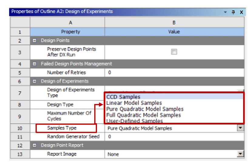
Figure 5 shows the sample points distributions of the optimal filling space design model.

Figure 5. Types of Sample Point Distribution in the Optimal Space-Filling Design Model

By selecting each of the models, software divides each input variable into several sample points. Now pay attention to the range of changes of each input parameter and calculate the difference between the upper and lower limit of each input variable and divide this difference by the number of points of the sample created. The value of this division is equal to the value of the distance between each of the points of the created sample with each other. If the number of generated sample points is numerically odd, the center sample point (middle value between maximum and minimum) is retained. This distance is periodically added to the top and bottom sides of this middle value until Reach the maximum, minimum range of that parameter.

If the number of generated sample points is even, ignore the center sample point (middle value between maximum and minimum) and add half of this distance to both sides and up and down this middle value to two points. Create in the middle of this interval and then add the full value of this distance periodically to the two midpoints up and down until it reaches the maximum and minimum interval of the parameter. For example, suppose an input parameter has a maximum and a minimum of 90 and 110, respectively.

An Example of The Optimal Space-Filling Design Model

By defining three input variables for the software and by using the optimal space-filling design method, the point distribution process of the sample points has been done by two methods of central composite design (CCD) and a full quadratic model. for example, by using the central composite design (CCD) sampling type, the number of segmented points for each input variable will be 15. As a result, we divide the distance between 90 and 110, equal to 20, by 15. They will be equal to 1.33. Also, since it is the number of odd points, keep the midpoint of this interval, which is 100.

This numerical distance equals Add 1.33 periodically to both sides of the number 100.

 

An Example in ANSYS Workbench

we have an example that the radius parameter has a range of changes from 90 mm to 110 mm. We have used the optimal space-filling design model and central composite design sampling type. For example, by using a full quadratic model, the number of segmented points for each input variable will be 10. As a result, we divide the distance between 90 and 110, equal to 20, by 10, equal to 2. Since the number of points is even, we calculate half the value of the calculated distance, the value of 1, to both sides of the midpoint of this interval.

We add the number 100 to produce the two midpoints of this interval equal to 101 and 99; we add this numerical distance equal to 2 to both sides of the numbers 101 and 99 periodically. We have an example that the radius parameter has a range of changes from 90 mm to 110 mm. Figure 6 shows the table created in the ANSYS Workbench software environment.

Figure 6. Distribution of Sample Points in the Optimal Space-Filling Method of Central Composite Design

DOE Models: Introducing the Custom Model

The special feature of this design model is that it allows the user to design the test design environment (DOE) as desired.  A table of input parameter values ​​is created when users enable the model instead of the default test environment (DOE). The user can enter the desired values ​​from the input parameters manually. Also, if users select another model of the test design before selecting this model, the same previously table remains on the screen. But users can change the values ​​in this table manually. Also, one of the other features of this design model is that users can call the external software files in CSV format to the table of design points.  User can see the ability to call external data to the software only when they select the custom design model.

Figure 7 shows a common design model with a sample (custom + sampling).

Figure 7. Distribution of Sample Points in the Conventional Design Model with a Sample with Two Input Parameters.

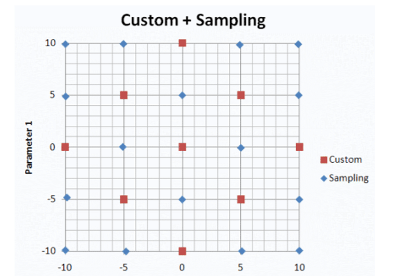
There are two ways to define design sample points manually. They include the custom model and the custom model with the sample (custom + sampling). Still, the difference between the two methods is that in the common model with the sample, users can determine the number of sample points (total number of samples) manually.

DOE Models: Sparse Grid Initialization Model

The sparse grid initialization model as a DOE model has three levels for dividing the various states of the input parameters. The three levels include -1, 0, +1, where levels +1 and -1 are equivalent to the maximum, and minimum of each input  parameter. Also, level 0 is equivalent to the mean value of that parameter. Therefore, this model divides each input factor into three parts or levels between its maximum and minimum values.

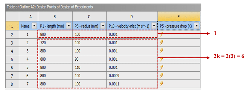
• k represents the number of input parameters or the same factors. The number 1 represents only the case where all factors have their middle value (same as level 0).
• The expression 2k indicates the cases in which each factor’s maximum and minimum value (same as level +1 or level -1).

An Example of The Sparse Grid Initialization Model

For example, suppose an input parameter has a maximum and a minimum of 90 and 110, respectively. Therefore, 90 and 110 represent level -1 and level +1, respectively. Also, the mean value of this interval, i.e., 100, also represents level 0.

There is an example that the radius parameter has a range of changes from 90 mm to 110 mm. Figure 8 shows the table created in the ANSYS Workbench software environment.

Figure 8. Table of Creative Design Points in an Example with Three Input Parameters by Central Composite Design Method.

Users should use this model when the goal is to create a sparse grid response surface. A scattered network response level is a model based on its desired accuracy. This type of response surface, where the gradient of the desired output parameters is higher, can automatically correct the matrix of design points to increase the accuracy of the response surface.

DOE Models: Latin Hypercube Sampling Design

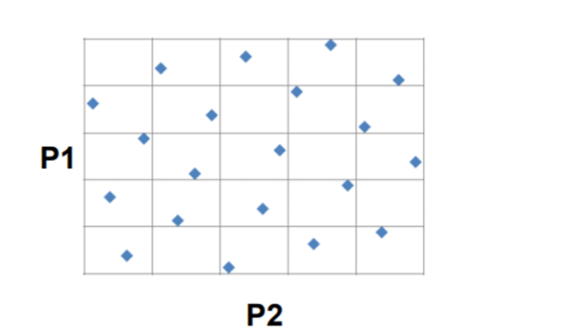
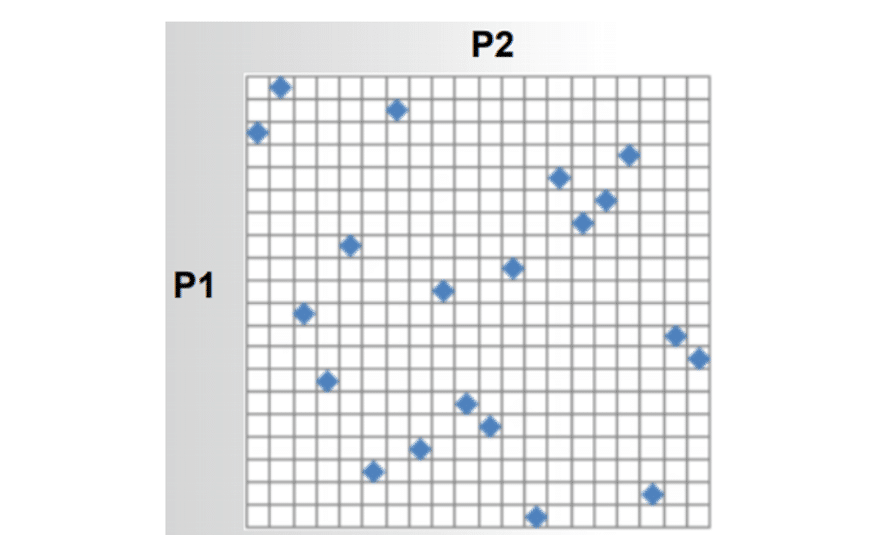
The Latin hypercube sampling design  is an advanced algorithm. This method  prevents the creation of sample points in a cumulative or clustered manner. This model, generates these points  randomly within each of the square grids in the design space, but users can find  two points  that have the same input parameter value.

Figure 9 shows the space containing the design points according to the Latin hypercube sampling design.

Figure 9. Distribution of Sample Points in the Latin Hypercube Sampling Model with Two Input Parameters

The Latin hypercube sampling design model also behaves like the optimal space-filling design in terms of how to select sample type points. The sample type selection methods are the same as the previous ones. The spacing process between the two sample points in the design space is the same as the previous method.The number of sample points for each input parameter and the amount of those sample points in both design models is similar. However, the layout of these sample design points differs between the defined input parameters in these two methods.