Finite Volume Method (FVM) in CFD

Description

Entering to FVM

Session 2 – Computational Fluid Dynamic Course

INTRODUCTION

Hello and welcome to second session of Computational Fluid Dynamic course by mister CFD team. In this session we are looking to enter Finite Volume Method field.

Let’s start with some simple examples and increase our knowledge of finite volume method approach of CFD to a level that from the next session enter the Fluent equations and methods.

EXAMPLE 1: HEAT TRANSFER IN A SOLID ROD

Problem Description:
The first problem that we are going to solve numerically is heat transfer in a solid rod. Consider a 1-dimensional rod that temperature at the one side of it is 20 degree of Celsius constant and temperature at the other end of rod is 100 degree of Celsius. The length of rod is 6 centimeter and the rod is very thin.

Transport Equation:

The general form of transport equation is presented here. For energy equation if we replace φ with internal energy that is specific heat multiply with temperature the following equation will resulted. Three source terms are added:
– First due to pressure gradient
– Second due to dissipation
– Last one is volume source term

Solution Method:

The rod is solid and also the problem is steady state. So, transient term, convection term, dissipation and pressure terms are zero and equation for pure diffusion will result.

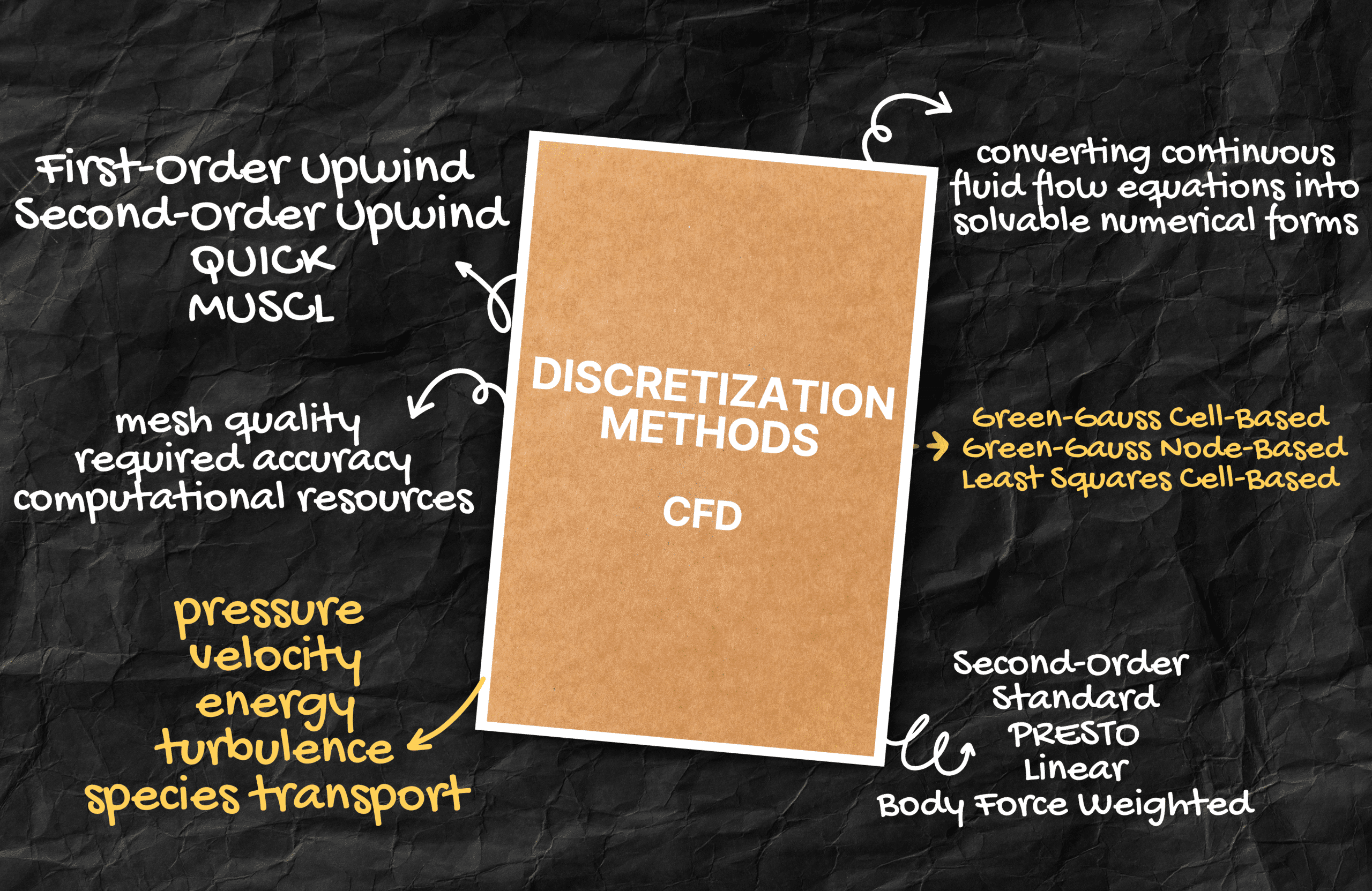
Discretization:

Now, let integrate equation over a control volume. By using Gauss’s divergence-theorem we can convert the volume integrate into a surface integrate of control volume boundaries.

Grid Generation:

The first step in the finite volume method is to divide the domain into discrete control volumes. Let us place a number of nodal points in the space between A and B. The boundaries (or faces) of control volumes are positioned mid-way between adjacent nodes. For this rod, it is divided into 6 control volumes.

Node Identification:

– A general nodal point is identified by P
– Neighbors in one-dimensional geometry: “nodes” to west (W) and east (E)
– West side face: lowercase w
– East side face: lowercase e
– Distances: delta x WP (between W and P), delta x PE (between P and E)
– Control volume width: delta x

DISCRETIZATION PROCESS

The discretized equation has a clear physical interpretation. This equation states that the diffusive flux of T leaving the east face minus the diffusive flux of φ entering the west face is equal to zero. It constitutes a balance equation for T over the control volume.

Interface Calculations:

For useful forms of discretized equations, we need:
– Interface thermal diffusion coefficient k
– Gradient of temperature respect to x at east (e) and west (w)

Uniform Grid Analysis:

Using Taylor series learned in the previous session, we can write value of thermal conductivity at nodes W and P with base point of w. By writing Taylor series till second term and truncating higher order terms, these relations result.

Cell Central Differencing:

By adding thermal diffusion at nodes P and W and divide by 2, thermal-diffusion at face w will calculate. Similarly for face e, using average of thermal diffusion at nodes P and E.

Temperature Calculations:

Writing temperature at point W and P in base of w with Taylor series till third term:
– First and third terms vanish
– Only derivative of T respect to x at w remains
– Similar process for derivative of T respect to x at e

Simplified Relations:

With constant thermal diffusion assumption:
– KE plus KP divided by two equals K
– Cross-section area cancels out
– Delta x is constant
Result: Temperature at point P is average of temperature at point East and West

Boundary Conditions:

– First and last nodes: Cannot use central scheme
– West face of first node: Forward discretization
– East face of last node: Backward discretization

MATRIX FORMULATION

Points numbered 1 to 6:
– Point 1: T1 = (2*20 + T2)/3
– Point 2: T2 = (T1 + T3)/2
[Continue with equations]

Solution Method:

– System solved using MATLAB
– Results shown in graph
– Comparison with analytical solution shows linear temperature change

EXAMPLE 2: COOLING OF A FIN

Problem Description:
Cylindrical fin with:
– Uniform cross-sectional area A
– Base temperature: 100°C
– Insulated end
– Ambient temperature: 20°C
– Convective heat transfer along length

Governing Equation:
Including:
– Heat transfer coefficient h
– Perimeter P
– Thermal conductivity k
– Ambient temperature T infinity

EXAMPLE 3: CHANNEL FLOW ANALYSIS

Problem Specifications:
– Channel length: 1 meter
– Width: 0.1 meter
– Inlet velocity: 5 m/s uniform
– Outlet condition: du/dx = 0
– Wall velocity: 0
– Assumption: zero y-velocity

Mathematical Formulation:
Starting from general transport equation, replacing φ with x-velocity for x-momentum equation. Steady state conditions apply.

CONCLUSION
In this session, we solved three examples using finite volume method:
1. Heat transfer in solid rod
2. Cooling fin analysis
3. Channel flow simulation

Next session will focus on governing equations and discretization methods used in Fluent software.