Internal Flow in pipe CFD Simulation, Different Flow Regimes, ANSYS Fluent
$120.00 $60.00 Student Discount
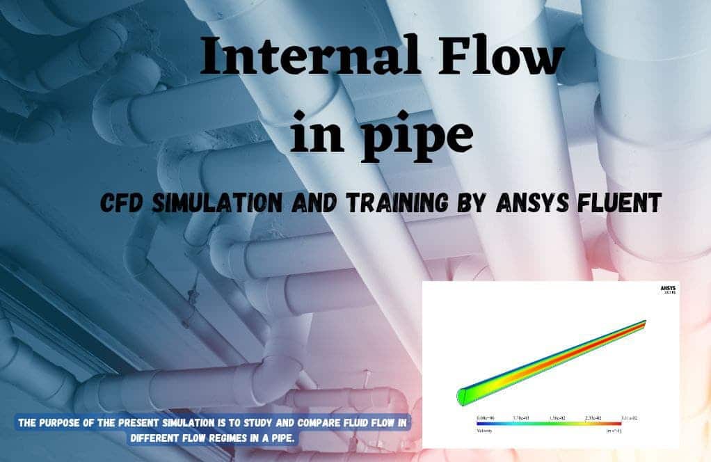
The purpose of the present simulation is to study and compare fluid flow in different flow regimes in a pipe.
Click on Add To Cart and obtain the Geometry file, Mesh file, and a Comprehensive ANSYS Fluent Training Video.To Order Your Project or benefit from a CFD consultation, contact our experts via email (info@mr-cfd.com), online support tab, or WhatsApp at +44 7443 197273.
There are some Free Products to check our service quality.
If you want the training video in another language instead of English, ask it via info@mr-cfd.com after you buy the product.
Description
Project Description of Internal Flow with Different Flow Regimes
The present problem simulates the internal flow of water through a simple horizontal pipe, which due to the symmetrical structure of this pipe, half of its geometry consists of a semi-cylinder has been studied by ANSYS Fluent. The purpose of the present simulation is to study and compare fluid flow in different flow regimes. For this purpose, this simulation is performed in three modes, which include laminar flow, k-Ԑ turbulence flow and k-ω turbulence flow. Laminar flow indicates the regular and uniform movement of fluid layers on top of each other and the absence of flow turbulence, including vortices.
Turbulent flow, on the other hand, indicates irregular motion of fluid particles with very large irregular vortices. To determine the type of flow regime, one must pay attention to the Reynolds number defined for the flow and compare its value with the critical Reynolds value in the mentioned geometric model. If the Reynolds number is greater than the critical Reynolds value, the flow is turbulent, and if the Reynolds number is less than the critical Reynolds value, it is laminar flow.
Project Description
Therefore, since the Reynolds number depends on the amount of flow inlet velocity, in the current simulation, the value of the inlet velocity is considered variable; So that for the first case, which is the laminar flow, the inlet flow velocity is considered to be 0.0176 m.s-1, and in the second and third cases, which are turbulent flow, the inlet flow velocity is considered to be 0.334 m.s-1. In general, laminar flow consists of solving one equation and turbulence flow consists of solving two equations.
The k-epsilon RNG turbulence model is used to model transient flows, flows in geometries with high curvatures, and air conditioning problems; While the k-omega standard turbulence model for modeling currents including velocity deceleration and separation due to reverse pressure gradient, mixing layer flows and plate and radial jets, high rotational flows, and issues related to aerodynamic forces and turbochargers are applicable.
Geometry & Mesh
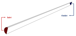
The 3-D geometry of the model is designed using Design Modeler software. The present model consists of a semi-cylinder with a radius of 0.015 m and a length of 1 m. The following figure shows a view of the graphic geometry.
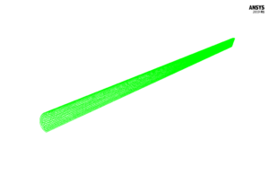
The meshing of the model has been done using ANSYS Meshing software and the mesh type is structured. The element number is 23120. The following figure shows the mesh.
CFD Simulation Setting of Internal Flow Considering Different Flow Regimes
To simulate the present model, several assumptions are considered:
- We perform a pressure-based solver.
- The simulation is steady.
- The gravity effect on the fluid is ignored.
A summary of the defining steps of the problem and its solution is given in the following table:
| Models | ||
| variable | Viscous model | |
| Boundary conditions | ||
| velocity inlet | Inlet | |
| 0.0167 m.s-1 for laminar | velocity magnitude | |
| 0.334 m.s-1 for turbulence | ||
| pressure outlet | Outlet | |
| 0 Pascal | gauge pressure | |
| Wall | Wall | |
| stationary wall | wall motion | |
| Solution Methods | ||
| SIMPLE | Pressure-velocity coupling | |
| Second order | pressure | Spatial discretization |
| Second order upwind | momentum | |
| Initialization (internal flow) |
||
| Standard | Initialization method | |
| 0 Pa | gauge pressure | |
| 0 m.s-1 | x-velocity , y-velocity | |
| 0.0167 m.s-1 for laminar | z-velocity | |
| 0.334 m.s-1 for turbulence | ||
Different Flow Regime Results
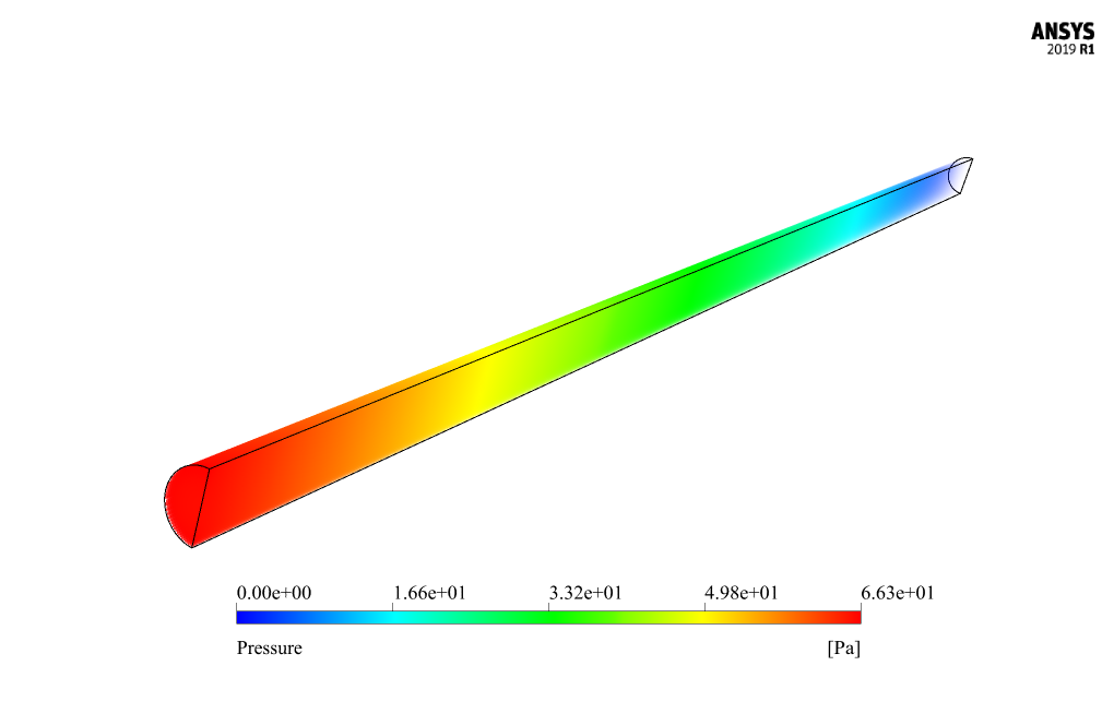
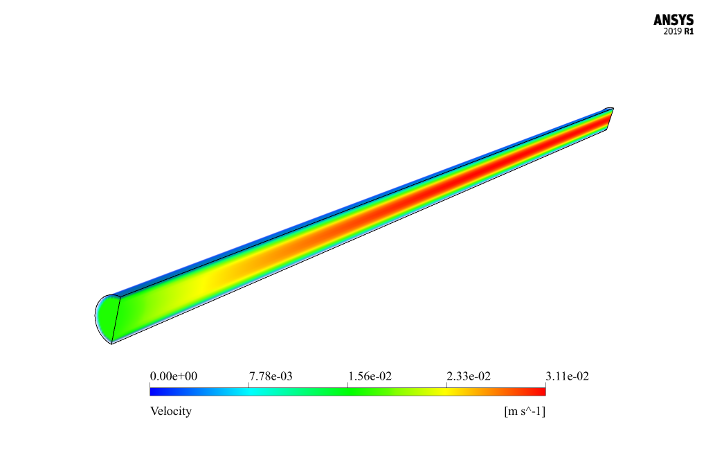
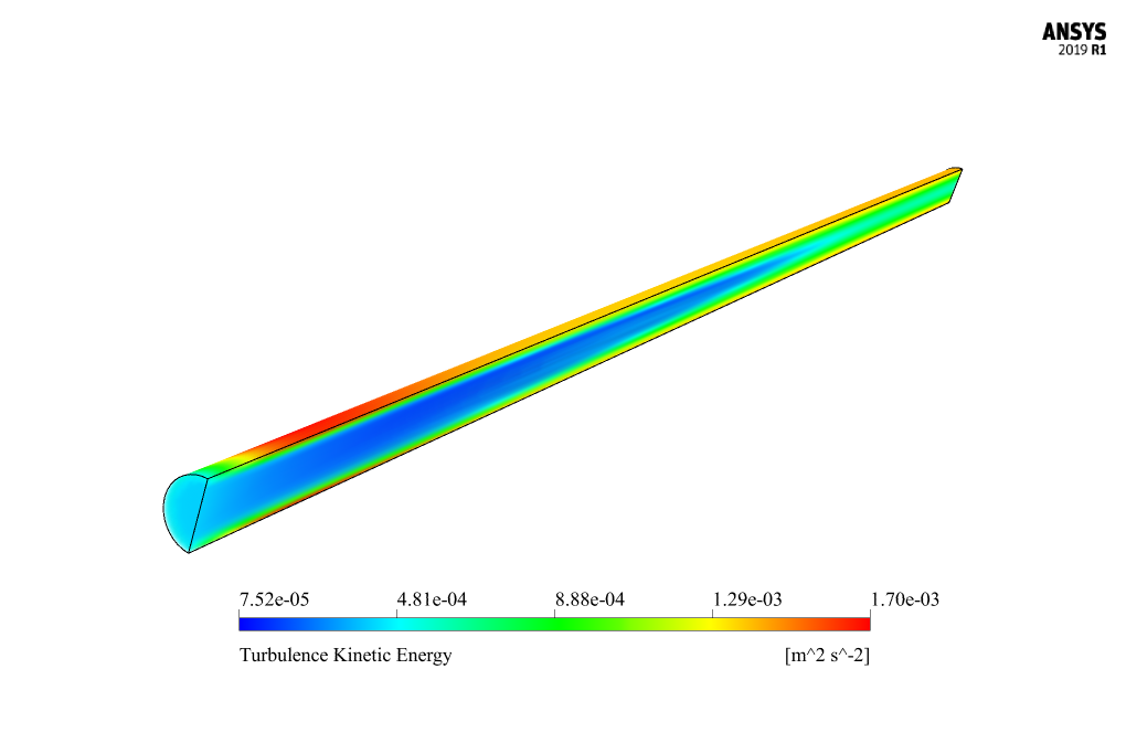
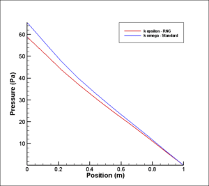
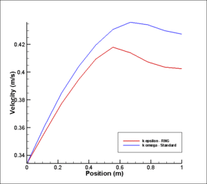
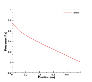
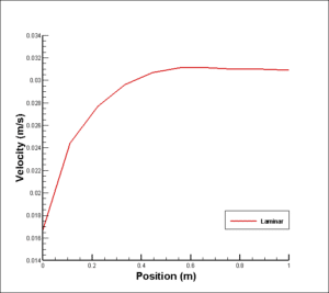
At the end of the solution process, we obtain two-dimensional and three-dimensional turbulence pressure, velocity and kinetic energy contours in three modes: laminar flow, k-epsilon RNG turbulence flow and k-omega standard turbulence flow. We display two-dimensional contours on the center plate of the pipe, which is a symmetrical plate. Also, we present velocity and pressure diagrams in terms of location in the central axis of the pipe for two different modes of turbulence flow.
Prof. Rex Hahn –
How are the results of the simulation visualized?
MR CFD Support –
The results are visualized using contour plots of pressure and velocity, as well as streamlines to show the fluid flow within the pipe.
Pink Russel –
Can this simulation be used to predict the pressure drop in a pipe?
MR CFD Support –
Absolutely! The results from this simulation can provide valuable insights into the pressure drop and velocity profile within the pipe.
Clarabelle Towne –
I am impressed by the level of detail in this simulation.
Darren Lesch –
I appreciate the commitment to accuracy and validation in this simulation.