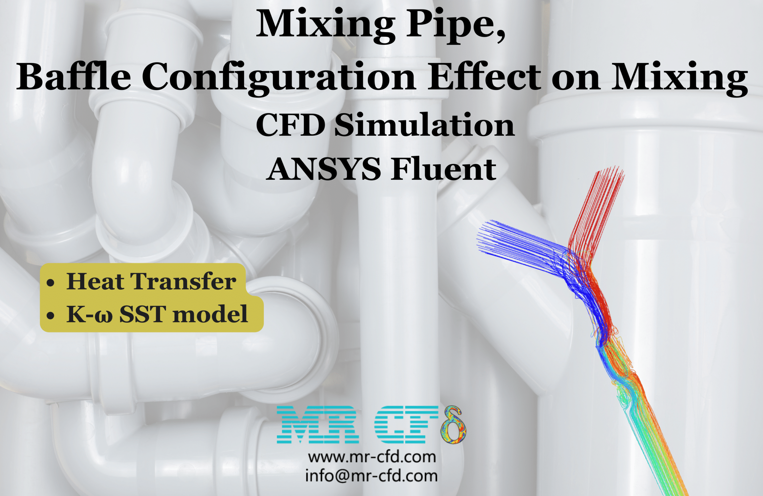
Mixing Pipe, Baffle Configuration Effect on Mixing, CFD Simulation
$80.00 $40.00 Student Discount
- The problem numerically simulates a mixing pipe, baffle configuration effect on mixing in ANSYS Fluent software.
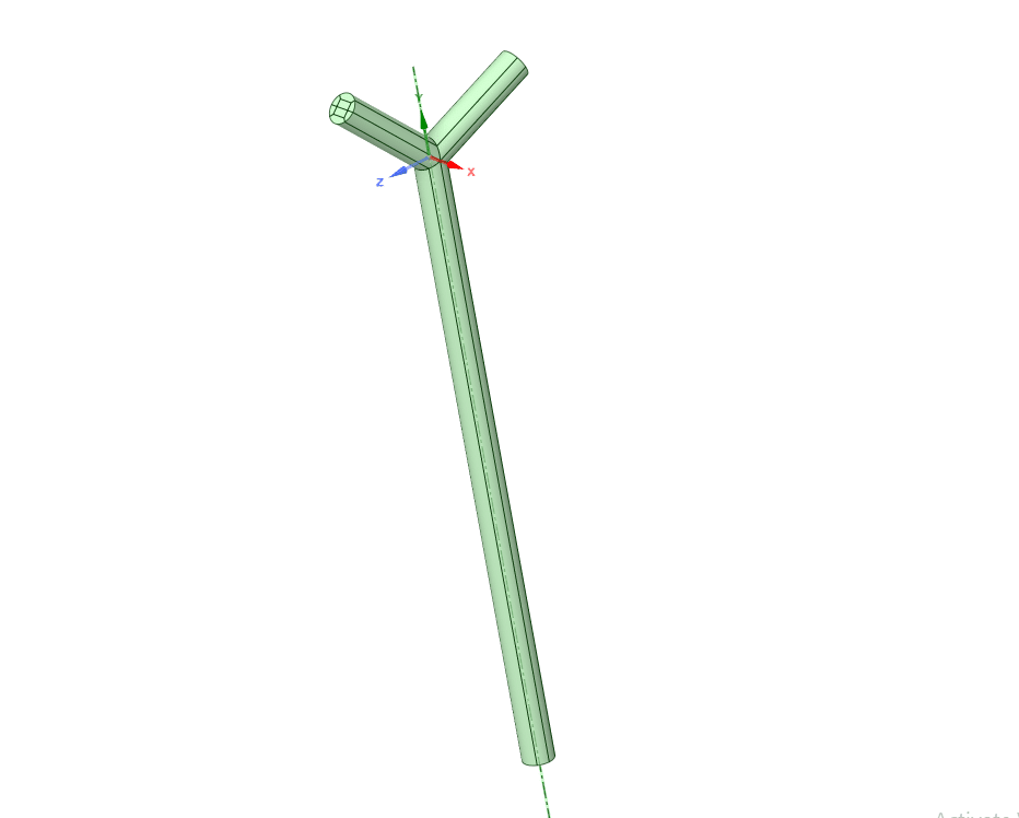
- The 3D geometry of the model is created in SpaceClaim software.
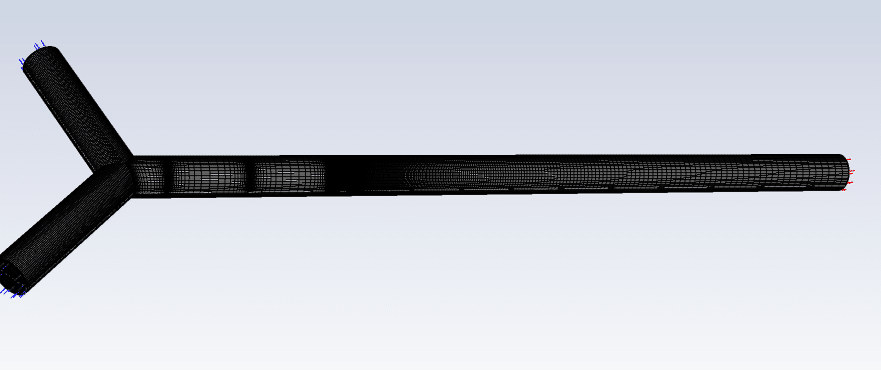
- The model is meshed in ANSYS Meshing creating structural mesh with 1,330,000 , 1,380,000 and 1,500,000 elements for the different cases.
- The K-ω SST model is used to describe turbulence of the flow.
To Order Your Project or benefit from a CFD consultation, contact our experts via email (info@mr-cfd.com), online support tab, or WhatsApp at +44 7443 197273.
There are some Free Products to check our service quality.
If you want the training video in another language instead of English, ask it via info@mr-cfd.com after you buy the product.
Description
Mixing Pipe, Baffle Configuration Effect on Mixing CFD Simulation Simulation, ANSYS Fluent
Description
In this project a mixing pipe with water flows in 2 high and low temperature is modeled in ANSYS Fluent Software. In this case, heat transfer occurs in two modes of conduction more likely near the boundary layer and convection in the main flow. The pipe wall is determined to be completely isolated and no heat loss or heat generation through the wall occurs.
High and low temperature water with 37 and 20 Celsius degree respectively come into a 10cm-diameter pipe inlets. Two pipes are joined with an angle of 90 degrees and the flow is mixed. It should be mentioned that the outlet conditions and mixing length depend on the velocities, temperatures, and geometry.
The geometry of the mixing pipe cases are designed in SpaceClaim and a structural mesh with 1,330,000 , 1,380,000 and 1,500,000 elements for the base case, 2-baffles case and 3-baffles case are generated in Ansys Meshing respectively.
Methodology
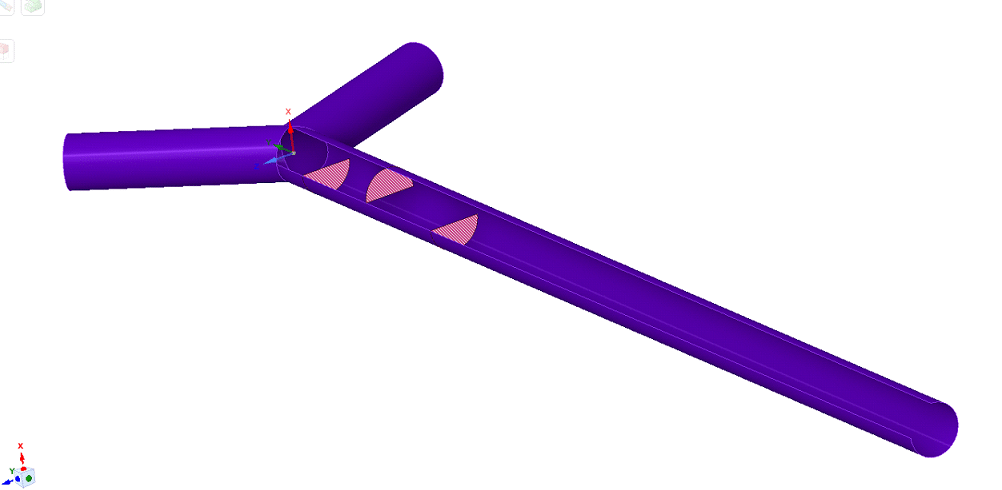
We are going to study the influence of the number and configuration of baffles on mixing the two flows via five cases: A base one that simply mixes two flow going out of the domain through the exit pipe,2 other cases with two and three baffles placed in the vertical configuration inside the pipe for better mixing and the last two cases with two and three baffles respectively in the horizontal configurations maximum y+ in this simulation is 2 and the average y+ is 0.25. The grid around the walls is fine enough so the turbulence model can catch viscous sublayer. The Reynolds of the inlet flows is 3000 so it is fully turbulent.
K-ω SST model was chosen for turbulence modeling because of the capability of this approach to model the mixing and secondary flows.
The inlet boundary condition of all cases are mass flow inlet with the same value so the only change between the two domains is the number and configuration of baffles.
Conclusion
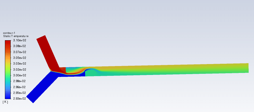
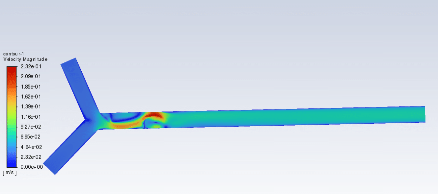
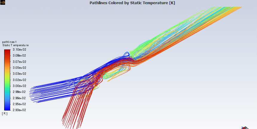
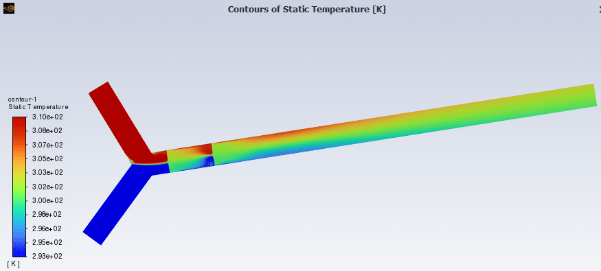
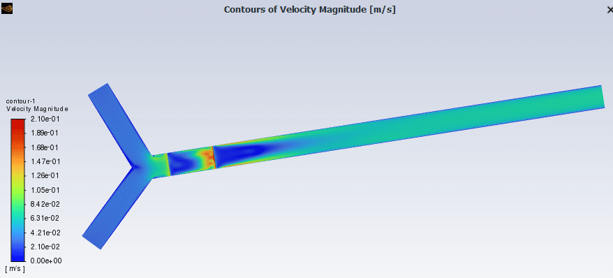
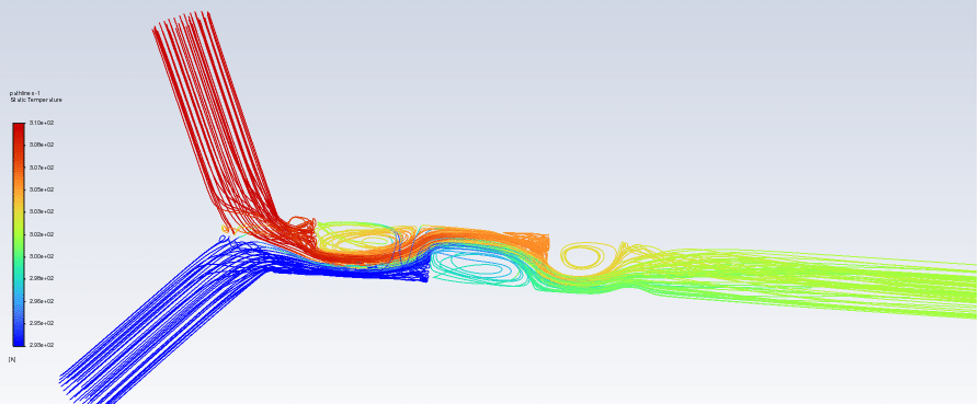
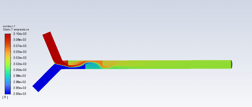
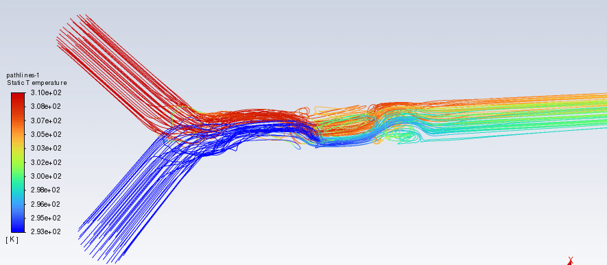
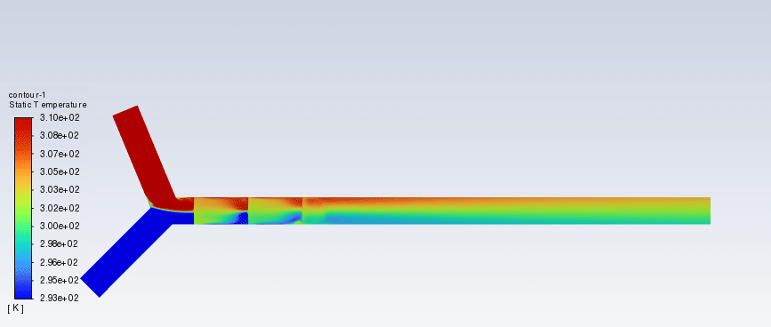
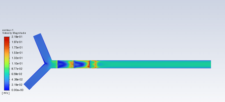
The velocity, temperature contours and Stream lines are reported along the pipe and across it so the flow behavior can be observed. Also Separation and secondary flow are obvious in the contours.
In the first case Flow is started to mix but at the end of the domain there is still nonuniformity in temperature and without using baffles flow needs longer pipe to mix properly.
In case 5 (3 horizontal baffles), the flow is detached behind the baffle’s wall and also at the joint of pipes. In this case at the end of the domain temperature is uniform and mixing is completed.
As the contours show at the exit of the base case there is still a 13-degree difference between the hot and cold zones of exit water. Adding baffle helps the mixing with any configuration but the horizontal configuration is more effective. The results are shown in the Table below.
| Case | Temperature non uniformity |
| Without baffle | 13.65 |
| 2 vertical baffles | 3.22 |
| 3 vertical baffles | 5.62 |
| 2 horizontal baffles | 3.1 |
| 3 horizontal baffles | 0.71 |





Reviews
There are no reviews yet.