Y-Plus Application in CFD Simulation

Introduction

The dimensionless variable Y-plus represents the distance from the wall to the first grid cell’s center, also, Y-plus is a distance with no dimensions. In other words, Y-plus renders the vertical space between the element’s center and the wall dimensionless, this value is used to evaluate the proportionality of the grid element’s size (height) on the wall boundaries.

On the other hand, the ratio of turbulent and laminar flow effects in a cell is represented by Y-plus. If Y-plus is low, the cell’s flow is laminar. If Y-plus is large, the current in that cell will be turbulent, As a result, if Y-plus is too small, then the flow in the cell is laminar slow, and the wall functions will not be usable.

We will explain how to work with Y-plus using the meshes we made in the following.

The Y-plus range for wall functions in ANSYS Fluent

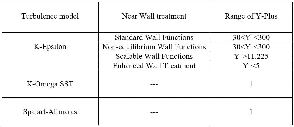
When using the wall function in Ansys Fluent, Y-plus should be specified in the range:

According to the table above, if the value of Y-plus is equal to 300, then we will use the K-Epsilon (Standard Wall Functions, Non-equilibrium Wall Functions, Scalable Wall Functions) turbulence model. If we have the value of Y-plus 1, we will use the K-Epsilon (Enhanced Wall Treatment), K-Omega SST, and Spalart-Allmaras.

practical example

To better understand what has been said, an attempt has been made to explain it in the form of a practical example done in ANSYS Fluent Software on naca0018 airfoil.

The turbulent flow around a naca0018 airfoil is simulated at a zero angle of attack. We will use the K-Epsilon (Standard Wall Functions, Non-equilibrium Wall Functions, Scalable Wall Functions), K-Epsilon (Enhanced Wall Treatment), K-Omega SST, Spalart-Allmaras turbulence models to solve this problem.

The law of the wall

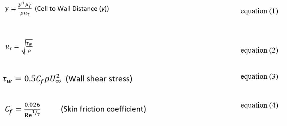
Viscosity and wall shear stress are important characteristics close to the wall. We define viscous scales, the suitable velocity and length scales in the near-wall area based on these variables.

Using equations 1 to 4, we can specify the cell to wall distance or the value y.

The initial and boundary conditions used in the present problem are as follows:

How to calculate the height of the cell adjacent to the wall corresponding to the value of Y-plus equal to 300

By placing this value in the above relations, the value of y is 0.006889.

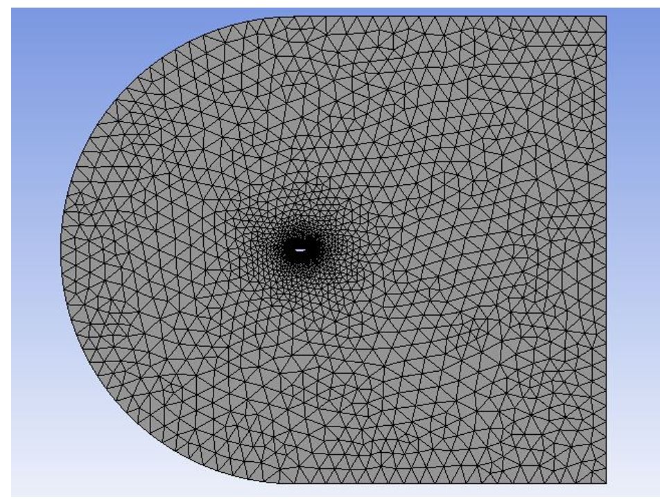
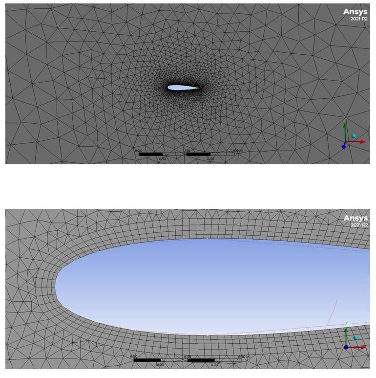
Simulations were run using the same mesh, material parameters, solver, and boundary conditions to illustrate the influence of the cell-based method. The area-averaged maximum and lowest values of Y-plus corresponded to the data mentioned above. The mesh that was utilized to y-plus=300 may be seen below.

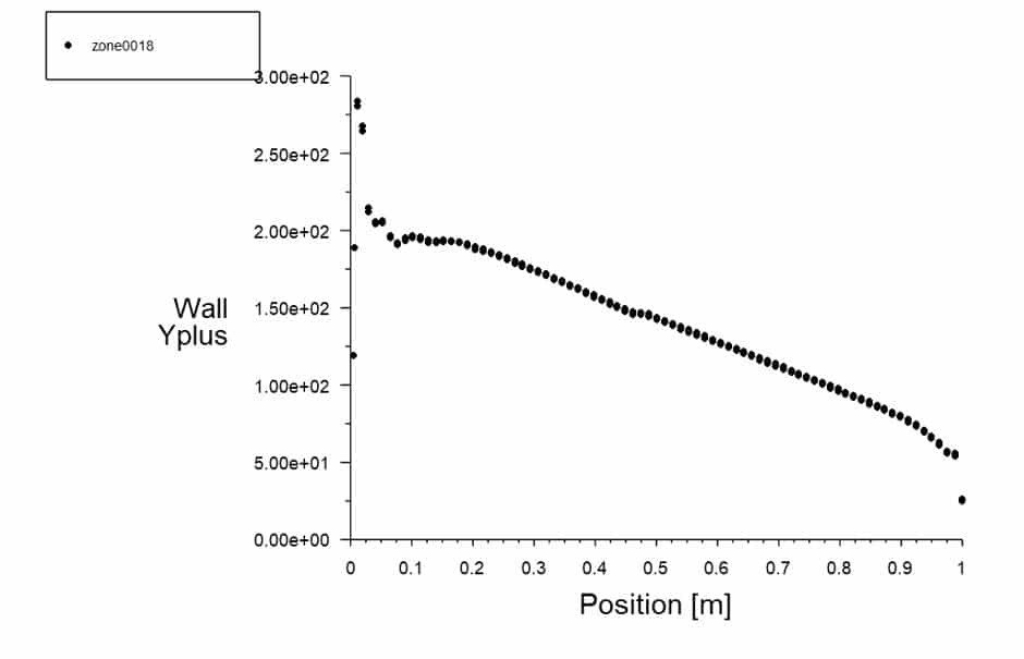
The value of Y-plus in fluent was printed for this case, which shows that the first layer height near-wall has been hit correctly:

As can be seen from the figure above, the Y-plus value ranges between 30 and 300.

By repeating the procedure for Y-plus 1, the value of y is 0.0000229, which indicates that the height value of the first layer becomes much smaller.

For the mesh to be of high quality, we must increase the number of boundary layers, or by using the Aspect Ratio, we can measure the last border layer with its neighboring mesh and not skip the mesh element.

 

How to calculate the height of the cell adjacent to the wall corresponding to the value of Y-plus equal to 1

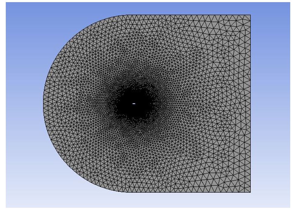
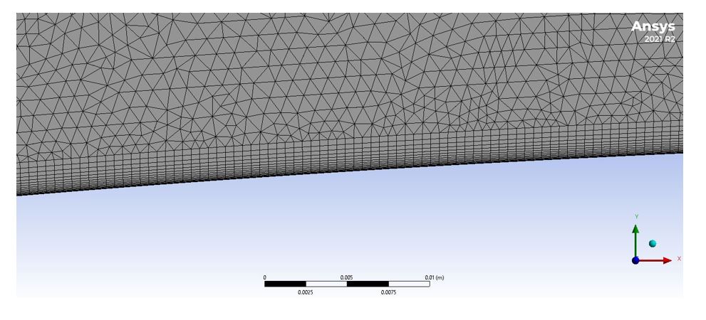
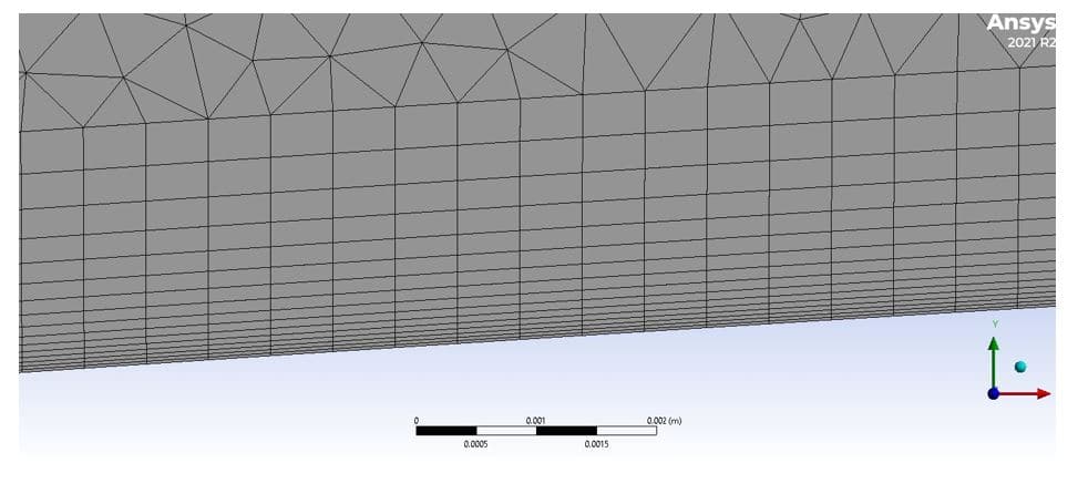
The mesh produced for Y-plus 1 is as follows; according to the figure, the number of mesh elements has increased compared to the previous state.

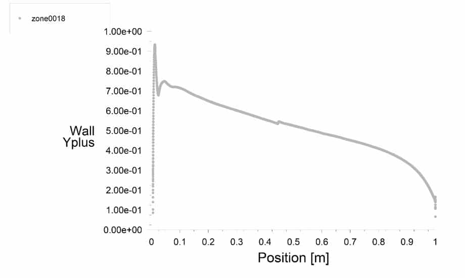
The value of Y-plus in fluent was printed for this case, which shows that the first layer height near-wall has been hit correctly:

As shown in the figure above, the Y-plus value is below 1.

Conclusion

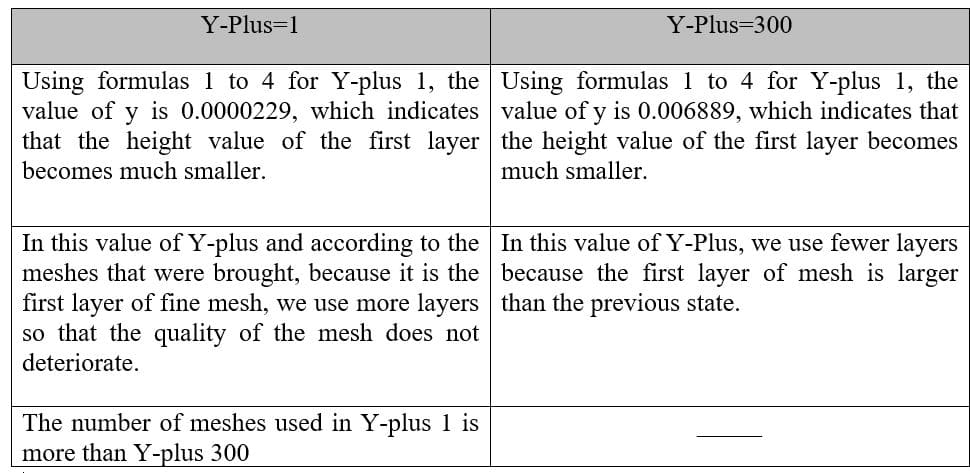
The table below shows the difference between Y-plus between 1 and 300: